Visualising Strategy Drawdowns

Along with the Sharpe Ratio, the drawdown of a trading strategy is one of the most common indicators you will see used to evaluate its performance. The drawdown is simply the decline in value of a strategy at a point in time since a previous high.

It's important as it gives you an indication of how painful the downside of a strategy could be, which is significant given people's tendency to avoid losses.

The drawdown usually takes into account two factors:

• The maximum drawdown magnitude - the maximum amount (expressed as a percentage), a strategy looses before returning to a previous high.
• The maximum drawdown duration - the maximum amount of time it takes for a strategy to return to a previous high.

As with all performance measures, it's useful to be able to visualise your maximum drawdowns. I'm going to show you how to generate the following chart showing you exactly that.

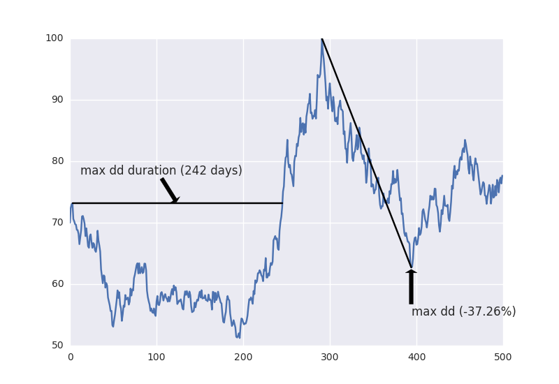
For simplicities sake our strategy is going long a stock who's prices follow a geometric Brownian motion path. We generate 500 daily price points, with a starting price of 70, annual returns ($\mu$) of 5% and standard deviations ($\sigma$) of 30%. We then calculate our cumulative returns (log returns could also be used) and PnL based on us being long this stock.

    start_price = 70.0
    prices = utils.generate_gbm_prices(500, 70.0, 0.05, 0.3, 1.0)
    returns = (utils.calculate_returns(prices) + 1.0).cumprod() - 1.0
    pnl = start_price * (returns + 1.0)

Where these functions are defined as:

DAYS_PER_YEAR = 252.0


def generate_gbm_prices(periods, start_price, mu, sigma, delta):
    t = delta / DAYS_PER_YEAR
    prices = np.zeros(periods)
    epsilon_sigma_t = np.random.normal(0, 1, periods-1) * sigma * np.sqrt(t)
    prices[0] = start_price
    for i in range(1, len(prices)):
        prices[i] = prices[i-1] * \
                    np.exp((mu - 0.5 * sigma**2) * t +
                           epsilon_sigma_t[i-1])
    return prices


def lag(data, empty_term=0.):
    lagged = np.roll(data, 1)
    lagged[0] = empty_term
    return lagged


def calculate_returns(prices):
    lagged_pnl = lag(prices)
    returns = (prices - lagged_pnl) / lagged_pnl

    # All values prior to our position opening in pnl will have a
    # value of inf. This is due to division by 0.0
    returns[np.isinf(returns)] = 0.
    # Additionally, any values of 0 / 0 will produce NaN
    returns[np.isnan(returns)] = 0.
    return returns

Next we calculate our maximum drawdowns - we require offsets for where the maximum drawdowns take place in order to plot them..

    max_dd, max_count, max_dd_idx, max_duration_idx, hwm_idx = \
        utils.calculate_max_drawdown(returns)

Where our drawdown function is defined as:

def calculate_max_drawdown(returns):
    size = len(returns)
    highwatermark = np.zeros(size)
    drawdown = np.zeros(size)
    dd_duration = np.zeros(size, dtype=int)

    for i in range(1, size):
        highwatermark[i] = max(highwatermark[i-1], returns[i])
        drawdown[i] = ((1.0 + returns[i]) / (1.0 + highwatermark[i])) - 1.0
        if drawdown[i] == 0.:
            dd_duration[i] = 0
        else:
            dd_duration[i] = dd_duration[i-1] + 1

    min_dd_idx = drawdown.argmin()
    return min(drawdown), max(dd_duration), \
           min_dd_idx, dd_duration.argmax(), \
           np.where(returns == highwatermark[min_dd_idx-1])[-1]

We can now generate the above plot of our returns with some nice labels of where our maximum drawdowns happen!

    plt.plot(pnl)
    plt.plot((hwm_idx, max_dd_idx),
             (pnl[hwm_idx], pnl[max_dd_idx]), color='black')
    plt.annotate('max dd ({0:.2f}%)'.format(max_dd * 100.0),
                 xy=(max_dd_idx, pnl[max_dd_idx]),
                 xycoords='data', xytext=(0, -50),
                 textcoords='offset points',
                 arrowprops=dict(facecolor='black', shrink=0.05))

    max_duration_start_idx = max_duration_idx - max_count
    max_duration_x1x2 = (max_duration_start_idx, max_duration_idx)
    max_duration_y1y2 = (pnl[max_duration_start_idx],
                         pnl[max_duration_start_idx])

    plt.plot(max_duration_x1x2, max_duration_y1y2, color='black')
    plt.annotate('max dd duration ({} days)'.format(max_count),
                 xy=((max_duration_start_idx + max_duration_idx) / 2,
                     pnl[max_duration_start_idx]),
                 xycoords='data',
                 xytext=(-100, 30), textcoords='offset points',
                 arrowprops=dict(facecolor='black', shrink=0.05))

    plt.show()

The full source code is listed below, and available here.

dd_example.py

import matplotlib.pyplot as plt
import numpy as np
import seaborn

import utils


np.random.seed(3)


def main():

    start_price = 70.0
    prices = utils.generate_gbm_prices(500, 70.0, 0.05, 0.3, 1.0)
    returns = (utils.calculate_returns(prices) + 1.0).cumprod() - 1.0
    pnl = start_price * (returns + 1.0)

    max_dd, max_count, max_dd_idx, max_duration_idx, hwm_idx = \
        utils.calculate_max_drawdown(returns)

    plt.plot(pnl)
    plt.plot((hwm_idx, max_dd_idx),
             (pnl[hwm_idx], pnl[max_dd_idx]), color='black')
    plt.annotate('max dd ({0:.2f}%)'.format(max_dd * 100.0),
                 xy=(max_dd_idx, pnl[max_dd_idx]),
                 xycoords='data', xytext=(0, -50),
                 textcoords='offset points',
                 arrowprops=dict(facecolor='black', shrink=0.05))

    max_duration_start_idx = max_duration_idx - max_count
    max_duration_x1x2 = (max_duration_start_idx, max_duration_idx)
    max_duration_y1y2 = (pnl[max_duration_start_idx],
                         pnl[max_duration_start_idx])

    plt.plot(max_duration_x1x2, max_duration_y1y2, color='black')
    plt.annotate('max dd duration ({} days)'.format(max_count),
                 xy=((max_duration_start_idx + max_duration_idx) / 2,
                     pnl[max_duration_start_idx]),
                 xycoords='data',
                 xytext=(-100, 30), textcoords='offset points',
                 arrowprops=dict(facecolor='black', shrink=0.05))

    plt.show()


if __name__ == '__main__':
    main()

utils.py

import numpy as np


DAYS_PER_YEAR = 252.0


def generate_gbm_prices(periods, start_price, mu, sigma, delta):
    t = delta / DAYS_PER_YEAR
    prices = np.zeros(periods)
    epsilon_sigma_t = np.random.normal(0, 1, periods-1) * sigma * np.sqrt(t)
    prices[0] = start_price
    for i in range(1, len(prices)):
        prices[i] = prices[i-1] * \
                    np.exp((mu - 0.5 * sigma**2) * t +
                           epsilon_sigma_t[i-1])
    return prices


def lag(data, empty_term=0.):
    lagged = np.roll(data, 1)
    lagged[0] = empty_term
    return lagged


def calculate_returns(prices):
    lagged_pnl = lag(prices)
    returns = (prices - lagged_pnl) / lagged_pnl

    # All values prior to our position opening in pnl will have a
    # value of inf. This is due to division by 0.0
    returns[np.isinf(returns)] = 0.
    # Additionally, any values of 0 / 0 will produce NaN
    returns[np.isnan(returns)] = 0.
    return returns


def calculate_max_drawdown(returns):
    size = len(returns)
    highwatermark = np.zeros(size)
    drawdown = np.zeros(size)
    dd_duration = np.zeros(size, dtype=int)

    for i in range(1, size):
        highwatermark[i] = max(highwatermark[i-1], returns[i])
        drawdown[i] = ((1.0 + returns[i]) / (1.0 + highwatermark[i])) - 1.0
        if drawdown[i] == 0.:
            dd_duration[i] = 0
        else:
            dd_duration[i] = dd_duration[i-1] + 1

    min_dd_idx = drawdown.argmin()
    return min(drawdown), max(dd_duration), \
           min_dd_idx, dd_duration.argmax(), \
           np.where(returns == highwatermark[min_dd_idx-1])[-1]

@misc{svensson2015-visualising-strategy-drawdowns,
  author = {Conor Svensson},
  title = {{Visualising Strategy Drawdowns}},
  year = {2015},
  month = mar,
  url = {https://conorsvensson.com/archive/quanttech/visualising-strategy-drawdowns/}
}